

Constant Acceleration Formula: 5 Equations, Derivations, and Worked Examples
The constant acceleration formula is v = v₀ + at, which gives the final velocity from the initial velocity, the acceleration, and the time. Four more equations link displacement, velocity, acceleration, and time. All 5 equations apply only when acceleration stays constant. Results are expressed in meters (m), meters per second (m/s), meters per second squared (m/s²), and seconds (s).
For a reliable reference, consult OpenStax section on acceleration.
What Is the Constant Acceleration Formula and What Are Examples of It?
The constant acceleration formulas are a set of 5 equations that describe motion in which velocity changes by equal amounts in equal time intervals. OpenStax University Physics Volume 1 presents these kinematic equations for motion along a straight line with constant acceleration. They are also called the kinematic equations, the SUVAT equations, and the uniformly accelerated motion equations.
Constant acceleration means the magnitude and the direction of the acceleration stay the same during the motion. The velocity-time graph of such motion is a straight line.
Examples of constant acceleration include free-falling objects near Earth's surface, cars that brake at a steady rate, carts on frictionless inclines, and objects pushed by a constant net force.
The table below defines each symbol in the constant acceleration formulas and lists its SI unit.
| Symbol | Meaning | SI Unit |
|---|---|---|
| Δx | Displacement (x − x₀) | meter (m) |
| x₀ | Initial position | meter (m) |
| x | Final position | meter (m) |
| v₀ | Initial velocity | m/s |
| v | Final velocity | m/s |
| a | Constant acceleration | m/s² |
| t | Elapsed time | second (s) |
| v_avg | Average velocity, equal to (v₀ + v) / 2 | m/s |
What Are the 5 Constant Acceleration Equations?
The 5 constant acceleration equations are v = v₀ + at, Δx = v₀t + ½at², Δx = vt − ½at², Δx = ½(v₀ + v)t, and v² = v₀² + 2aΔx. Each equation leaves out 1 of the 5 variables (Δx, v₀, v, a, t). The table below lists the equations, the variable each one omits, and the known quantities each one uses.
| No. | Equation | Variable Not Included | Known Quantities |
|---|---|---|---|
| 1 | v = v₀ + at | Displacement (Δx) | v₀, a, t |
| 2 | Δx = v₀t + ½at² | Final velocity (v) | v₀, a, t |
| 3 | Δx = vt − ½at² | Initial velocity (v₀) | v, a, t |
| 4 | Δx = ½(v₀ + v)t | Acceleration (a) | v₀, v, t |
| 5 | v² = v₀² + 2aΔx | Time (t) | v₀, a, Δx |
The position form of equation 2 is x = x₀ + v₀t + ½at². Equation 5 is also written as v² = v₀² + 2a(x − x₀).
How Do You Solve a Constant Acceleration Problem Step by Step?
A constant acceleration problem is solved by listing 3 known variables, naming the unknown, and selecting the equation that omits the remaining variable. The 7 steps are:
- Choose a positive direction and assign signs to all vectors.
- List the 3 known variables with units.
- Name the unknown variable.
- Identify the variable that is neither known nor requested.
- Select the equation that omits that variable.
- Solve for the unknown and check the units and the sign.
- Verify the result with a second equation.
Example: A train slows from 30 m/s to 10 m/s over 400 m. The known variables are v₀ = 30 m/s, v = 10 m/s, and Δx = 400 m.
- Time is not involved in the acceleration, so equation 5 applies: a = (v² − v₀²) / (2Δx) = (100 − 900) / 800 = −1 m/s².
- Acceleration is not involved in the time, so equation 4 applies: t = 2Δx / (v₀ + v) = 800 / 40 = 20 s.
- The check with equation 1 gives v = 30 + (−1)(20) = 10 m/s, which matches.
How Do You Choose the Right Constant Acceleration Formula?
The right formula is the equation that omits the variable that is neither given nor requested. The table below lists the 5 omitted variables and the matching equation.
| Variable Not Involved | Equation to Use |
|---|---|
| Displacement (Δx) | v = v₀ + at |
| Final velocity (v) | Δx = v₀t + ½at² |
| Initial velocity (v₀) | Δx = vt − ½at² |
| Acceleration (a) | Δx = ½(v₀ + v)t |
| Time (t) | v² = v₀² + 2aΔx |
Phrases in a problem signal the known values. The phrase "starts from rest" gives v₀ = 0. The phrase "comes to a stop" gives v = 0. The phrase "dropped" gives v₀ = 0 and a = g. The phrase "at the top of its flight" gives v = 0 for the vertical motion.
How Do You Rearrange the Constant Acceleration Formulas?
Each equation rearranges to solve for any variable it contains. The table below lists 11 rearranged forms for acceleration, velocity, time, and displacement.
| Unknown | Formula | Known Quantities |
|---|---|---|
| a | a = (v − v₀) / t | v₀, v, t |
| a | a = 2(Δx − v₀t) / t² | Δx, v₀, t |
| a | a = (v² − v₀²) / (2Δx) | v₀, v, Δx |
| v | v = v₀ + at | v₀, a, t |
| v | v = √(v₀² + 2aΔx) | v₀, a, Δx |
| v₀ | v₀ = v − at | v, a, t |
| v₀ | v₀ = √(v² − 2aΔx) | v, a, Δx |
| t | t = (v − v₀) / a | v₀, v, a |
| t | t = 2Δx / (v₀ + v) | Δx, v₀, v |
| Δx | Δx = (v² − v₀²) / (2a) | v₀, v, a |
| Δx | Δx = v_avg × t | v₀, v, t |
Square-root forms give 2 mathematical roots. The sign of the velocity follows the direction of motion at that moment.
What Are 5 Worked Examples of the Constant Acceleration Formulas?
Each of the 5 equations solves a different combination of known quantities. The table below lists the known quantities, the equation, the calculation, and the result for 5 problems.
| No. | Known Quantities | Unknown | Equation | Calculation | Result |
|---|---|---|---|---|---|
| 1 | v₀ = 10 m/s, a = 2 m/s², t = 5 s | v | v = v₀ + at | 10 + 2 × 5 | 20 m/s |
| 2 | v₀ = 5 m/s, a = 3 m/s², t = 4 s | Δx | Δx = v₀t + ½at² | 5 × 4 + ½ × 3 × 16 | 44 m |
| 3 | v = 30 m/s, a = 2 m/s², t = 5 s | Δx | Δx = vt − ½at² | 30 × 5 − ½ × 2 × 25 | 125 m |
| 4 | v₀ = 8 m/s, v = 20 m/s, t = 6 s | Δx | Δx = ½(v₀ + v)t | ½ × 28 × 6 | 84 m |
| 5 | v₀ = 0, v = 30 m/s, Δx = 90 m | a | a = (v² − v₀²) / (2Δx) | 900 / 180 | 5 m/s² |
Checks confirm the results. Example 2 gives v = 5 + 3 × 4 = 17 m/s, and (17² − 5²) / (2 × 3) = 44 m. Example 3 gives v₀ = 30 − 2 × 5 = 20 m/s, and ½ × (20 + 30) × 5 = 125 m. Example 5 gives t = 30 / 5 = 6 s, and ½ × 30 × 6 = 90 m.
How Are the Constant Acceleration Formulas Derived?
The formulas are derived by integrating the definition of acceleration (a = dv/dt) with a constant value of a. The 5 steps are:
- Start with a = dv/dt and integrate with respect to time: v = v₀ + at.
- Integrate the velocity: x = x₀ + v₀t + ½at², which gives equation 2.
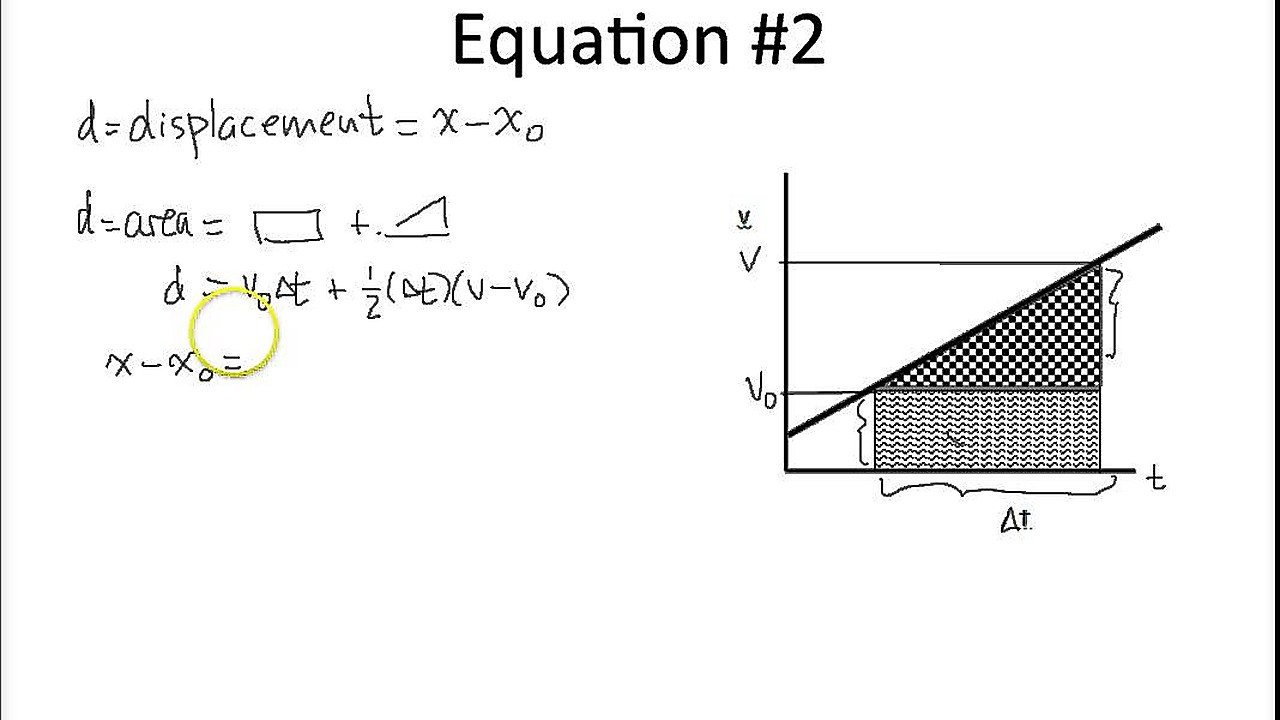
- Use the average velocity of a straight-line velocity graph, v_avg = (v₀ + v) / 2, to obtain equation 4: Δx = ½(v₀ + v)t.
- Substitute v₀ = v − at into equation 2 to obtain equation 3: Δx = vt − ½at².
- Substitute t = (v − v₀) / a into equation 4 to obtain equation 5: Δx = (v² − v₀²) / (2a).
Galileo Galilei showed in Two New Sciences in 1638 that the distance covered from rest grows with the square of time. The Oxford Calculators at Merton College stated the mean speed theorem in the 1330s, which is the basis of equation 4.
How Do You Find Time When the Equation Is Quadratic?
Time is found by solving the quadratic equation ½at² + v₀t − Δx = 0 with the quadratic formula. The formula is t = (−v₀ ± √(v₀² + 2aΔx)) / a. The positive root that follows the start of the motion gives the answer.
Example with 1 valid root: v₀ = 4 m/s, a = 2 m/s², and Δx = 21 m.
- The discriminant is 4² + 2 × 2 × 21 = 100.
- The roots are (−4 + 10) / 2 = 3 s and (−4 − 10) / 2 = −7 s.
- The root −7 s lies before the start, so t = 3 s.
- The check gives 4 × 3 + ½ × 2 × 9 = 21 m.
Example with 2 valid roots: v₀ = 10 m/s, a = −2 m/s², and Δx = 21 m.
- The equation becomes t² − 10t + 21 = 0.
- The roots are t = 3 s and t = 7 s.
- The object passes 21 m at 3 s with a velocity of +4 m/s, and again at 7 s with a velocity of −4 m/s.
- The maximum displacement is 25 m, reached at t = 5 s.
How Do You Use the Constant Acceleration Formulas for Braking and Stopping Distance?
Stopping distance is found with Δx = v₀² / (2a), where a is the magnitude of the deceleration. The formula comes from equation 5 with v = 0. The stopping time is t = v₀ / a.
The table below lists 5 initial speeds with a deceleration of 7 m/s² and no reaction time. The stopping distance is calculated with Δx = v₀² / 14.
| Initial Speed (km/h) | Initial Speed (m/s) | Stopping Distance (m) | Stopping Time (s) |
|---|---|---|---|
| 30 | 8.33 | 4.96 | 1.19 |
| 50 | 13.89 | 13.78 | 1.98 |
| 80 | 22.22 | 35.27 | 3.17 |
| 100 | 27.78 | 55.12 | 3.97 |
| 120 | 33.33 | 79.37 | 4.76 |
Doubling the speed multiplies the stopping distance by 4, as the rows for 50 km/h and 100 km/h show. A reaction time of 1.0 s adds v₀ × 1.0 s of travel at constant speed, which equals 27.78 m at 100 km/h. The total distance is then 55.12 + 27.78 = 82.90 m.
How Do the Constant Acceleration Formulas Apply to Free Fall?
Free fall is constant acceleration with a = g = 9.8 m/s² directed downward, if air resistance is absent. NIST defines standard gravity as exactly 9.80665 m/s². The table below lists 4 times for an object dropped from rest, with downward as the positive direction.
| Time (s) | Speed (v = gt) in m/s | Distance Fallen (Δy = ½gt²) in m |
|---|---|---|
| 1 | 9.8 | 4.9 |
| 2 | 19.6 | 19.6 |
| 3 | 29.4 | 44.1 |
| 4 | 39.2 | 78.4 |
Example for an upward throw: A ball leaves the hand at 20 m/s upward, with upward as positive and a = −9.8 m/s².
- The velocity at the top is 0, so the time to the top is 20 / 9.8 = 2.04 s.
- The maximum height is 20² / (2 × 9.8) = 20.41 m.
- The flight time back to the release point is 2 × 2.04 = 4.08 s.
- The landing speed is 20 m/s downward.
Example for a cliff: An object dropped from 45 m reaches the ground after t = √(2 × 45 / 9.8) = 3.03 s with a speed of 9.8 × 3.03 = 29.7 m/s.
The table below lists the surface gravity of 3 bodies and the fall time from rest over 2 m, calculated with t = √(2h / g).
| Body | Surface Gravity (m/s²) | Fall Time Over 2 m (s) |
|---|---|---|
| Earth | 9.8 | 0.64 |
| Moon | 1.62 | 1.57 |
| Mars | 3.71 | 1.04 |
In 1971, Apollo 15 commander David Scott dropped a hammer and a feather on the Moon. Both reached the surface at the same time, because the Moon has no air resistance.
How Do the Constant Acceleration Formulas Apply to Projectile Motion?
Projectile motion splits into a horizontal part with zero acceleration and a vertical part with a = −g. The horizontal equation is x = v₀ cos θ × t. The vertical equations are v_y = v₀ sin θ − gt and y = v₀ sin θ × t − ½gt².
Example: A ball launches at 20 m/s and 30° above the horizontal on level ground.
- The horizontal velocity is 20 × cos 30° = 17.32 m/s.
- The initial vertical velocity is 20 × sin 30° = 10 m/s.
- The time of flight is 2 × 10 / 9.8 = 2.04 s.
- The maximum height is 10² / (2 × 9.8) = 5.10 m.
- The range is 17.32 × 2.04 = 35.35 m.
How Do You Write the Constant Acceleration Formulas in 2 Dimensions?
The vector forms are v⃗ = v⃗₀ + a⃗t and Δr⃗ = v⃗₀t + ½a⃗t². Each component follows its own equation, so the x-axis and the y-axis are solved separately.
Example: v⃗₀ = (3, 4) m/s and a⃗ = (2, −1) m/s² act for t = 2 s.
- Final velocity: (3 + 2 × 2, 4 − 1 × 2) = (7, 2) m/s.
- Displacement: (3 × 2 + ½ × 2 × 4, 4 × 2 − ½ × 1 × 4) = (10, 6) m.
- Displacement magnitude: √(10² + 6²) = 11.66 m.
- Final speed: √(7² + 2²) = 7.28 m/s.
How Do You Read Constant Acceleration From Graphs?
Constant acceleration appears as a horizontal line on an acceleration-time graph, a straight sloped line on a velocity-time graph, and a parabola on a position-time graph. The table below lists each graph with its shape and the meaning of its slope and area.
| Graph | Shape for Constant Acceleration | Meaning of the Slope | Meaning of the Area |
|---|---|---|---|
| Acceleration-time | Horizontal line | 0, because a does not change | Change in velocity (Δv) |
| Velocity-time | Straight sloped line | Acceleration (a) | Displacement (Δx) |
| Position-time | Parabola | Instantaneous velocity at that point | Not used |
Example: A velocity-time line rises from 5 m/s at 0 s to 17 m/s at 4 s.
- Slope: (17 − 5) / 4 = 3 m/s²
- Area of the trapezoid: ½ × (5 + 17) × 4 = 44 m
- Area on the acceleration-time graph: 3 × 4 = 12 m/s, which equals the change in velocity
Beichner published a study of kinematics graph interpretation in the American Journal of Physics in 1994. The study found that students have difficulty interpreting the area under a velocity-time graph.
How Do You Know if Acceleration Is Constant?
Acceleration is constant when the velocity changes by equal amounts in equal time intervals. 3 checks confirm constant acceleration:
- Velocity check: equal time steps produce equal velocity changes.
- Graph check: the velocity-time graph is a straight line.
- Position check: the second differences of position at equal time steps are constant and equal a × Δt².
The table below shows data for v₀ = 2 m/s and a = 2 m/s², with a time step of 1 s.
| Time (s) | Position (m) | Velocity (m/s) | Velocity Change Per 1 s (m/s²) |
|---|---|---|---|
| 0 | 0 | 2 | Not applicable |
| 1 | 3 | 4 | 2 |
| 2 | 8 | 6 | 2 |
| 3 | 15 | 8 | 2 |
| 4 | 24 | 10 | 2 |
The position changes are 3, 5, 7, and 9 m. The second differences equal 2 m, which equals 2 × 1².
What Is the Difference Between Constant Velocity, Constant Acceleration, and Changing Acceleration?
Constant velocity has zero acceleration, constant acceleration has a fixed nonzero value, and changing acceleration has a value that varies with time. The table below compares the 3 types by 5 features.
| Feature | Constant Velocity | Constant Acceleration | Changing Acceleration |
|---|---|---|---|
| Acceleration | 0 | Fixed nonzero value | Varies with time |
| Velocity-time graph | Horizontal line | Straight sloped line | Curve |
| Position-time graph | Straight sloped line | Parabola | Higher-order curve |
| Displacement formula | Δx = vt | 5 kinematic equations | Δx = ∫ v(t) dt |
| Example | A cruise-control car on a straight road | A dropped stone in vacuum | A skydiver approaching terminal velocity |
Example of changing acceleration: a(t) = 6t + 4 with v₀ = 0 gives v(t) = 3t² + 4t. At t = 2 s, the velocity is 20 m/s and the displacement is 16 m. The constant acceleration equation gives a different, incorrect result.
What Are the Limits of the Constant Acceleration Formulas?
The formulas apply only when acceleration stays constant during the whole interval. 6 conditions limit them:
- Air resistance: drag grows with speed, so acceleration decreases. A skydiver reaches a terminal speed in the range of 50 to 60 m/s.
- Varying forces: springs and magnetic forces change the acceleration with position.
- Changing mass: rockets lose mass, so acceleration changes at constant thrust.
- Circular motion: the direction of the acceleration vector changes continuously.
- Multi-stage motion: each stage with a different acceleration requires its own calculation.
- Relativistic speeds: motion near the speed of light requires relativistic kinematics.
Split a multi-stage motion at each change of acceleration. The final velocity of stage 1 becomes the initial velocity of stage 2.
What Are the Units of the Constant Acceleration Formulas and How Are They Converted?
The SI unit of acceleration is meters per second squared (m/s²). The table below lists 4 acceleration units and 3 velocity units with their values in SI units.
| Quantity | Unit | Value in SI Units |
|---|---|---|
| Acceleration | Foot per second squared (ft/s²) | 0.3048 m/s² |
| Acceleration | Standard gravity (g) | 9.80665 m/s² |
| Acceleration | Mile per hour per second (mph/s) | 0.44704 m/s² |
| Acceleration | Kilometer per hour per second (km/h/s) | 0.27778 m/s² |
| Velocity | Kilometer per hour (km/h) | 0.27778 m/s |
| Velocity | Mile per hour (mph) | 0.44704 m/s |
| Velocity | Foot per second (ft/s) | 0.3048 m/s |
Divide km/h by 3.6 to obtain m/s. Example: A car accelerates from 0 to 100 km/h in 8 s. The final velocity is 27.78 m/s, and the acceleration is 27.78 / 8 = 3.47 m/s², which equals 0.35 g.
How Do You Measure Constant Acceleration Experimentally?
Constant acceleration is measured by recording the distance and the time of a cart released from rest and applying a = 2Δx / t². Instruments include stopwatches, photogates, motion detectors, and smartphone accelerometers. The 5 steps are:
- Set a cart on a ramp with a measured length.
- Release the cart from rest.
- Record the travel time with a stopwatch or photogate.
- Calculate a = 2Δx / t².
- Repeat 3 trials and average the results to reduce random error.
Example: A cart travels 1.2 m in 2.0 s. The acceleration is 2 × 1.2 / 2.0² = 0.6 m/s². On a frictionless incline, a = g sin θ, so sin θ = 0.6 / 9.8 and θ ≈ 3.5°.
How Do the Constant Acceleration Formulas Compare With the Rotational Formulas?
The rotational formulas have the same structure, with angular quantities in place of linear quantities. They apply when the angular acceleration (α) is constant. The table below pairs each linear equation with its angular form.
| Linear Equation | Angular Equation |
|---|---|
| v = v₀ + at | ω = ω₀ + αt |
| Δx = v₀t + ½at² | Δθ = ω₀t + ½αt² |
| Δx = vt − ½at² | Δθ = ωt − ½αt² |
| Δx = ½(v₀ + v)t | Δθ = ½(ω₀ + ω)t |
| v² = v₀² + 2aΔx | ω² = ω₀² + 2αΔθ |
Example: A wheel starts from rest with α = 5 rad/s² for 4 s. The angular velocity is 5 × 4 = 20 rad/s. The angular displacement is ½ × 5 × 16 = 40 rad, which equals 6.37 revolutions.
What Are Real-Life Applications of the Constant Acceleration Formulas?
The formulas apply to 6 fields. Examples include vehicle braking, aircraft takeoff, ballistics, free-fall timing, crash reconstruction, and spacecraft engine burns. The table below lists 4 calculations.
| Application | Known Quantities | Unknown | Equation | Result |
|---|---|---|---|---|
| Aircraft takeoff run | v₀ = 0, v = 70 m/s, a = 3 m/s² | Δx and t | v² = v₀² + 2aΔx and v = v₀ + at | 816.7 m and 23.3 s |
| Emergency braking | v₀ = 25 m/s, v = 0, a = −8 m/s² | Δx | Δx = (v² − v₀²) / (2a) | 39.06 m |
| Rifle barrel | v₀ = 0, v = 400 m/s, Δx = 0.6 m | a | a = (v² − v₀²) / (2Δx) | 133,333 m/s² |
| Cliff drop | v₀ = 0, Δy = 45 m, a = 9.8 m/s² | t and v | Δy = ½at² and v = at | 3.03 s and 29.7 m/s |
Crash investigators use skid length with a measured deceleration to estimate the speed before braking, through v₀ = √(2aΔx).
What Are the Common Mistakes When Using the Constant Acceleration Formulas?
7 common mistakes cause incorrect results. Research by David Trowbridge and Lillian McDermott, published in the American Journal of Physics in 1981, found that introductory physics students commonly have difficulty distinguishing acceleration from velocity.
The mistakes include:
- Applying the formulas to motion with changing acceleration.
- Dropping the sign of a deceleration.
- Mixing units, such as km/h for velocity with seconds for time.
- Treating zero velocity as zero acceleration.
- Ignoring the second root of a quadratic equation.
- Using distance in place of displacement when the motion reverses.
- Skipping the sign convention for upward and downward motion.
Example of the fourth mistake: A ball thrown upward has v = 0 at the top of its flight, and the acceleration is still −9.8 m/s². The velocity changes sign at that point.
What Do People Also Ask About the Constant Acceleration Formula?
What is the constant acceleration formula?
The basic formula is v = v₀ + at, which gives the final velocity from the initial velocity, the acceleration, and the time.
What are the 5 kinematic equations?
The 5 equations are v = v₀ + at, Δx = v₀t + ½at², Δx = vt − ½at², Δx = ½(v₀ + v)t, and v² = v₀² + 2aΔx.
What is the formula for displacement with constant acceleration?
The formula is Δx = v₀t + ½at², which uses the initial velocity, the acceleration, and the time.
What is the constant acceleration formula without time?
The formula is v² = v₀² + 2aΔx, which uses the initial velocity, the final velocity, the acceleration, and the displacement.
What is the constant acceleration formula without final velocity?
The formula is Δx = v₀t + ½at².
What is the constant acceleration formula without acceleration?
The formula is Δx = ½(v₀ + v)t, which uses the average velocity.
What is constant acceleration?
Constant acceleration is acceleration that keeps the same magnitude and direction during the whole motion.
What is the unit of constant acceleration?
The SI unit is meters per second squared (m/s²).
Is gravity a constant acceleration?
Gravity produces a constant acceleration of about 9.8 m/s² near Earth's surface, if air resistance is absent.
Can velocity be zero while acceleration is constant and not zero?
Velocity is zero at the top of a thrown ball's flight, while the acceleration stays at −9.8 m/s².
What does a constant acceleration graph look like?
The velocity-time graph is a straight sloped line, and the position-time graph is a parabola.
Do the formulas work for deceleration?
The formulas work for deceleration when the acceleration carries a negative sign along the direction of motion.
How do you find time with constant acceleration?
Use t = (v − v₀) / a, or t = 2Δx / (v₀ + v) if acceleration is unknown.
What is the stopping distance formula?
The stopping distance is Δx = v₀² / (2|a|), which comes from v² = v₀² + 2aΔx with v = 0.
When do the constant acceleration formulas not apply?
The formulas do not apply when the acceleration changes, as with air drag, springs, and rockets that lose mass.
What Is the Constant Acceleration Formula and How Is It Applied?
The constant acceleration formula is v = v₀ + at, which gives the final velocity in m/s. The 5 equations link displacement, initial velocity, final velocity, acceleration, and time, and each equation omits 1 of the 5 variables. Selecting the equation that omits the variable that is neither known nor requested solves any problem with 3 known values. The equations apply when acceleration stays constant, and the velocity-time graph is a straight line with a slope equal to a. Applications include braking distance, aircraft takeoff, free fall, projectile motion, ballistics, and rotating wheels.
Title: Definition of Newton's Second Law of Motion: Formula, 3 Forms, and Worked Examples

The University of the West Indies
My passion as a teacher and leader in education is to contribute to students’ enhanced learning by creation of a positive teaching/learning environment, where they are motivated to develop strong critical thinking, analytical and problem-solving skills.
As acting Vice-Principal and head of Physics, I have amassed five years of experience in leading meetings, implementing strategies to maintain discipline and school ethos, liaise with stakeholders in planning for future development of the institution; successfully negotiated the implementation of various projects for student development as well as supervising effective execution of such. For the past 19 years, I have incorporated discovery learning within the classroom through practical activities, problem solving and cooperative learning and have realized that students retention in Physics and Mathematics have increased significantly.
I am always cognizant that students have different learning styles, and as such teaching strategies during planning and delivery must take this crucial factor into consideration and be tailored to meet such differences.